Is the Rascal dead?

Short answer: At least until 2017, maybe forever. I'm teaching freshman engineering at Tufts University this fall. In conjunction with my efforts at raising a 3-year-old, this means the Rascal is on hold.

Long answer: First, a quick summary of the history. I started the design of the original Rascal in April of 2010 and sold the first run of 15 production units in January of 2012. After a few hardware tweaks in small batches of ~20 units in 2012, I made larger runs of ~100 units in late 2012 and 2013 while I worked on the software. I also designed the Precision Voltage Shield, started manufacturing it here in Somerville, and selling it alongside the Rascal.

Around the same time, I worked on a couple of interactive public art projects with public artists Dan Sternof Beyer and Bevan Weissmann. In the winter of 2012-2013, Dan and I made the giant lightblades on Boston's Greenway controllable by text messages. In the summer, I built the electronic guts of the Culture Tap kiosks that Dan and Bevan installed on Tremont Street in Boston.

In late 2013, my daughter was born, which shifted my view of life tremendously. I went from wanting to build my own Rascal Micro embedded systems empire to just wanting to do satisfying engineering work with a schedule flexible enough to raise my daughter well. As Chris Rogers, my colleague at Tufts, said to me, "Yeah, when you have kids, that's when you start thinking."

I announced the Rascal 2 in 2014 and made a batch of 10 prototypes. At the same time, I also founded a second company with Dan, Bevan, and 2 other friends of mine: New American Public Art.

I also worked on a number of short consulting projects with friends of mine:

• a new, lighter version of the TD-1B chain tensioner for holding aircraft onto carriers for the US Navy
• an analytics dashboard for a wind turbine company
• a wireless data acquisition system for recording data from inside tank treads for the US Army
• Built in mid 2014: Blue Hour in Camden, New Jersey

At some point in 2015, I discovered that someone in China was selling lousy A/D boards under my product's name, "Precision Voltage Shield". The unfortunate part is that they used a lamer chip, so it only gives 12 bits of precision, which is the same as the Arduino Due and the Arduino Zero. They also used bare male pins for the input lines, which is a step down from the screw terminals I used, but whatever. Have fun shorting out your board anyway.

That was exciting for me-- someone thought my product was good enough to want to take the name! (If I had to name the board again, I think I'd pick something different; I'd probably call it an Analog Input Shield, because that's the term the Arduino folks use.)

In parallel, sales of the Rascal started to flag. I had already announced the Rascal 2, and compared to all the other cheaper, faster boards available now, the original Rascal is slow and underpowered (though still easier to use, I would argue).

In 2015 and 2016, New American Public Art really started taking off. In the winter, we rebuilt Blue Hour for a light festival in Baltimore in March. This was followed by one of most ambitious installations, Ourself in Camden, New Jersey.

Finally, in 2016, I was offered a job at Tufts teaching freshman how to make stuff. I had intended to keep selling Rascals and Precision Voltage Shields, but as I was preparing to teach the class this summer, I started getting support emails about a board that is electrically quite similar to the Precision Voltage Shield, but cheaper. (Maybe it's not electrically identical, as the Precision Voltage Shield works, and, at least from the emails I got, this one seems not to. On the other hand, their satisfied customers would not be emailing support.) This left me with a dilemma-- do I want to try to compete with the folks undercutting me or not?

Ian MacKaye, a founder of Dischord Records, talks about how he wants to make the number of records that people want to buy. If 1000 people want a record, he wants to press 1000 copies, not 10,000 or 100. I feel the same way about my business. If the world demand for Precision Voltage Shields is sopped up by these boards from China, great. I have no interest in trying to flog the universe with advertising to get people to buy something from me. I'd rather find a new problem worth solving.

So that's where I stand. I'm going to teach this class at Tufts; after that, I'll probably build a new Rascal, if no more compelling problem needs solving.

Also, hello to all you Tufts students. I see you googling me.

A sleuth pursues a mysterious Rascal 2 bug

The upper deck on the Rascal 2 will have a Freescale Kinetis MK20 processor on it, so it can act like a Arduino, or a Teensy 3.1, or a Fadecandy. (The Teensy 3.1 uses the same chip, and the Fadecandy is almost identical, but with slightly less memory.) To prototype this, I've been building a demo that involves a Rascal 2 brain (the Beaglebone Black, hereafter BBB) talking to a Fadecandy. The Fadecandy will run an animation of flames on some WS2812 LED strips.

I got the Fadecandy working with BBB as a preliminary test a few months ago. Then, a couple days ago, I pull out a new BBB and try plugging in the Fadecandy. Curiously, the board shuts down after around 10 seconds. Since the power LED goes out, it looks like the power management chip is detecting a fault and cutting power. I unplug the Fadecandy and reboot. The BBB still shuts down after 10 seconds or so. No matter how many times I reboot the board, even with nothing attached, it shuts down a couple of seconds after reaching a login prompt.

Time to call on un1tz3r0.

I head over to un1tz3r0's sublair, inside Blake's secret lair. (Here's Blake's lair during the construction of the Penrose Triangle in 2013.)

After I eat one of his jelly doughnuts, Z3r0 pulls out a Fadecandy and BBB that he had from some LED art project. We set them up on his bench with a Samsung phone charger supplying the power. I'm a bit skeptical of the power supply, but I don't say anything because Z3r0 gave me a jelly doughnut and who am I to complain?

Z3r0's setup works immediately. We see, in dmesg, something like this:

[    1.276945] usb 1-1: skipped 1 descriptor after interface
[    1.277044] usb 1-1: default language 0x0409
[    1.277357] usb 1-1: udev 2, busnum 1, minor = 1
[    1.277373] usb 1-1: New USB device found, idVendor=1d50, idProduct=607a
[    1.277385] usb 1-1: New USB device strings: Mfr=1, Product=2, SerialNumber=3
[    1.277396] usb 1-1: Product: Fadecandy
[    1.277406] usb 1-1: Manufacturer: scanlime
[    1.277416] usb 1-1: SerialNumber: IAHO-ROTCIV-ONIDNOC
[    1.277878] usb 1-1: usb_probe_device
[    1.277895] usb 1-1: configuration #1 chosen from 1 choice
[    1.278006] usb 1-1: adding 1-1:1.0 (config #1, interface 0)
[    1.278360] usb 1-1: adding 1-1:1.1 (config #1, interface 1)
[    1.278811] hub 1-0:1.0: state 7 ports 1 chg 0000 evt 0002
[    1.278845] hub 1-0:1.0: port 1 enable change, status 00000103

So what's wrong with my setup?

Piece by piece, we replace each element of his system with mine. My Fadecandy works with his BBB. We add my USB cable, and it still works. Finally, all my stuff is working, using just his power supply. That suggests that the problem was my power supply back at the Asylum, but that's unlikely because I was running off the Rascalfarm, so at least 4 other Rascals are running on the same power bus, and they've all been working fine for months.

Z3r0 lets me borrow his power supply (OK, be honest, it's just a USB phone charger), just in case, and I head back to the Asylum. I thank him for his assistance and doughnut, and he vanishes into his lair (and sublair). It is 35 and raining. In New England, we call this "spring."

Back at the Asylum, I plug the working system into the Rascalfarm power supply. My understanding of the universe is piped to /dev/null as the system shuts down after 10 seconds. I wonder whether Z3r0's doughnut was laced with something. This is insane. All the other boards in the Rascalfarm are still running off the same 5 V supply.

I switch to Z3r0's power supply, and the damn thing starts working again, so now I know that the problem must be the power supply. When I measure the voltage, the problem is revealed: the supply voltage is sagging 0.5 V between the power supply output and the Rascalfarm power connector. The effect of this is that the first 4 boards work fine, but when the 5th board tries to boot, it can't quite get the juice it needs at the 10 second mark. (I'm not sure exactly what subsystem is being turned on then.)

Here's what's going wrong:

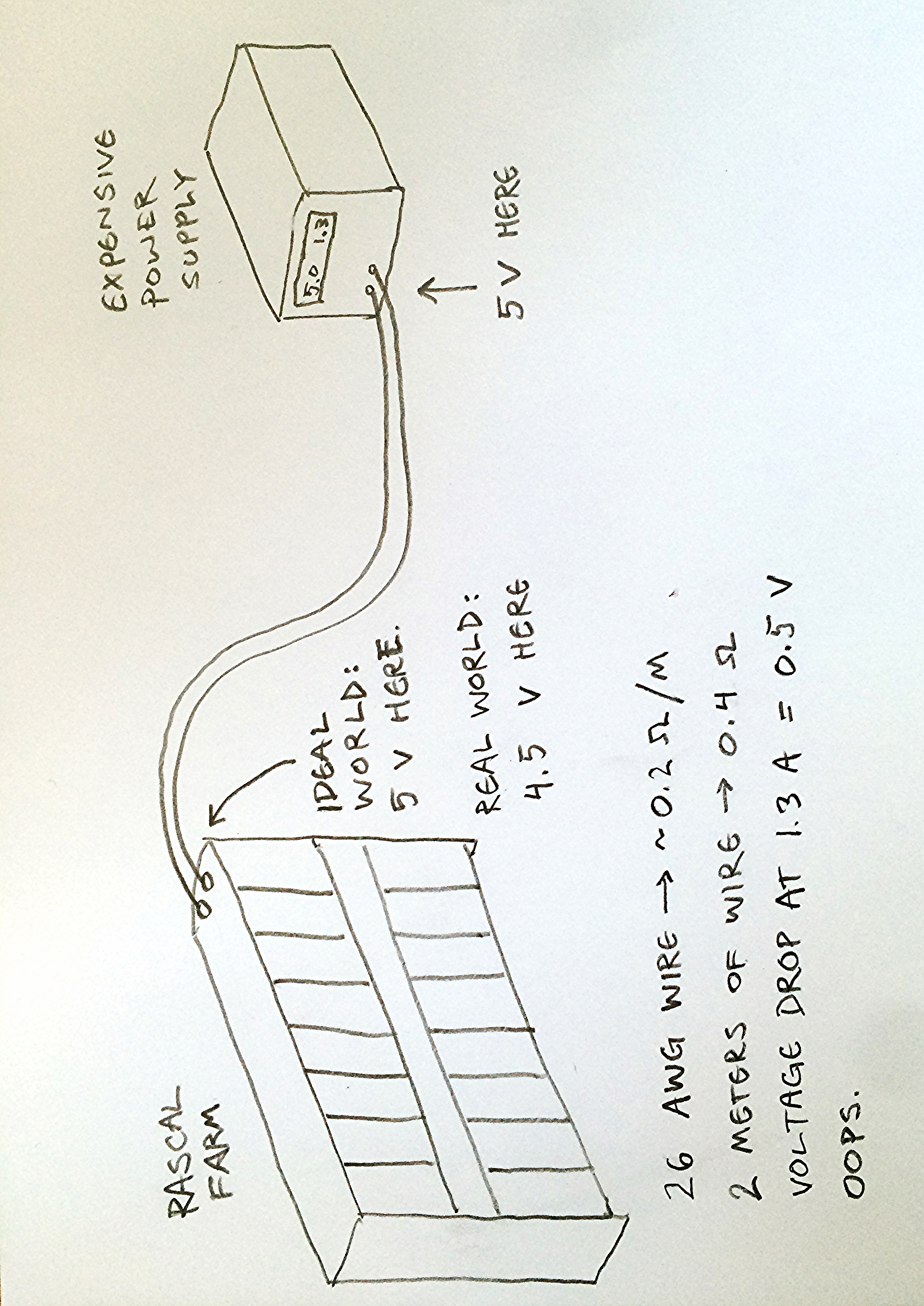
When I boost the power supply up to 5.5 V to compensate for the sagging, everything starts working.

My power supply may be a high-precision beauty, but even it is subject to Ohm's law.

Epilogue

This morning, I rewired the Rascalfarm with fat, low-resistance wire. Problem solved.

Thanks for the doughnut, Z3r0.

Building the Rascalfarm

Working with embedded Linux boards like the Raspberry Pi, or Beaglebone, you will fairly quickly realize that the hardware is far more polished than the software. It's not too surprising-- the boards are sold with the expectation that you will program the board to make it do what you want. Usually, the base software is just a Linux kernel with some hardware-specific drivers and basic Unix utilities added. I've found that some of the Linux kernels released crash as frequently as every couple of hours.

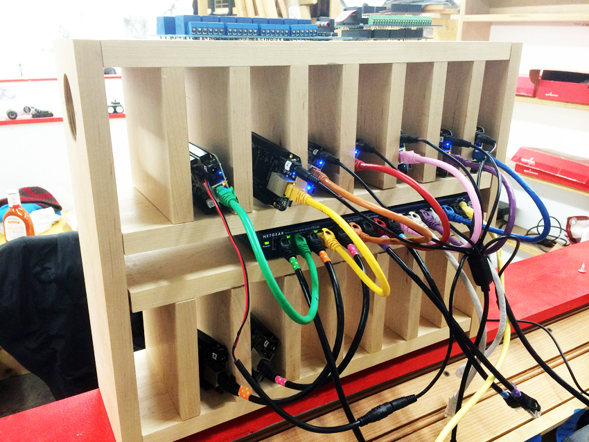
I'm now basing the Rascal on top of the Beaglebone Black hardware, so I needed a way to test the software in a more rigorous way than just, "Hey, this thing doesn't seem to have crashed while I was paying attention to it." To that end, I've been working on a rack of 15 Rascals that report over the network to a syslog server every time they reboot. In the long run, they will also emit a heartbeat signal that is monitored by a simple microcontroller on the rack. If one of the Rascals misses a couple of heatbeats, the microcontroller assumes the Rascal is dead and cycles the power to that board.

Revision 1: a crappy prototype

My first attempt was just a maple 1x6 I scored during a makerspace cleanup a few months back. I sliced the board up into 2 shelves and 14 dividers. I used a pin nailer to attach the dividers to the base.

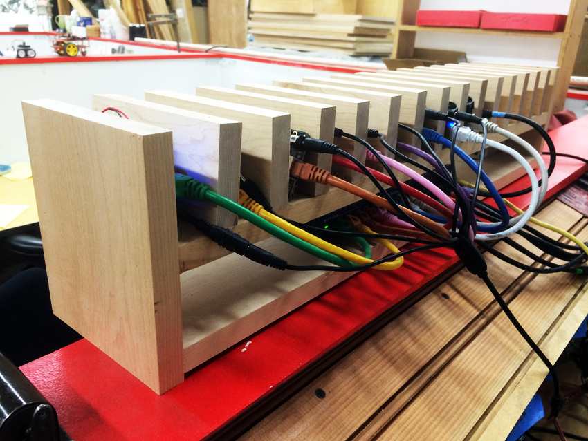
It's hard to discern on the lower shelf, but the rainbow of Ethernet cables is plugged into a 16 port switch.

Rev 1 was marginally functional, but it had a few problems: it took up a lot of space on my desk, the Ethernet cables I had didn't quite span the slots, and the dividers were really wobbly. But hey, it only took an hour or two to make.

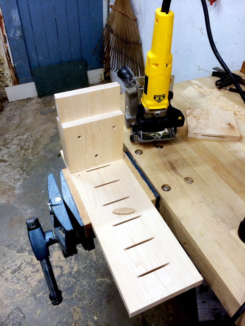
Revision 2: would you like a biscuit?

To stiffen up the dividers, I switched to wooden biscuit joints. I also reshaped the rack into two stacked rows of Rascals with the Ethernet switch in between. This also shortened the average cable span so that all the Ethernet cables reached.

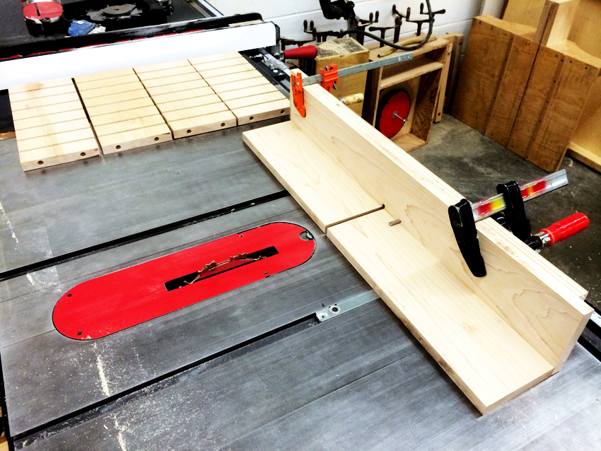
I cut the biscuit slots using a biscuit joiner in my basement. Each biscuit was spaced from the previous one as it was cut with a 1.522" +/- 0.010" spacer block. The picture below shows the first divider and spacer in place. The major weakness of this design is that the errors in position accumulate from slot to slot. One of the levels came out beautifully, but the second one was off by around 0.100" by the last divider. I hadn't done much woodworking with hard maple before, so I didn't realize that this much error would look sloppy in the end. With pine, I could have just clamped the bejesus out of everything, and it would look fine (though not exactly square).

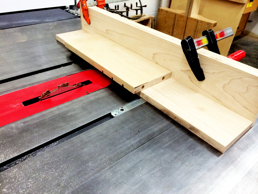
(Here are the slots with the biscuits inserted.)

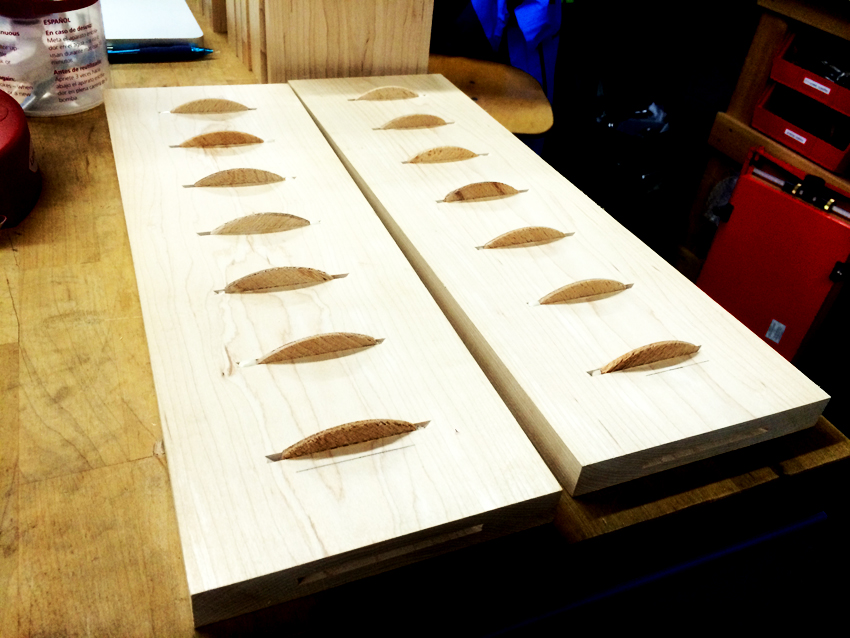
The second revision was decent-- it took up less desk space, it was extremely rigid, and all the cables reached their targets. Unfortunately, the gaps in the joints annoyed me every time I looked at the Rascalfarm. The power wiring was also still messy.

The second revision also let me test the Arduino and relay system for power cycling. I wired the relays so that they are normally closed, so if the Arduino hangs, the Rascals can keep running.

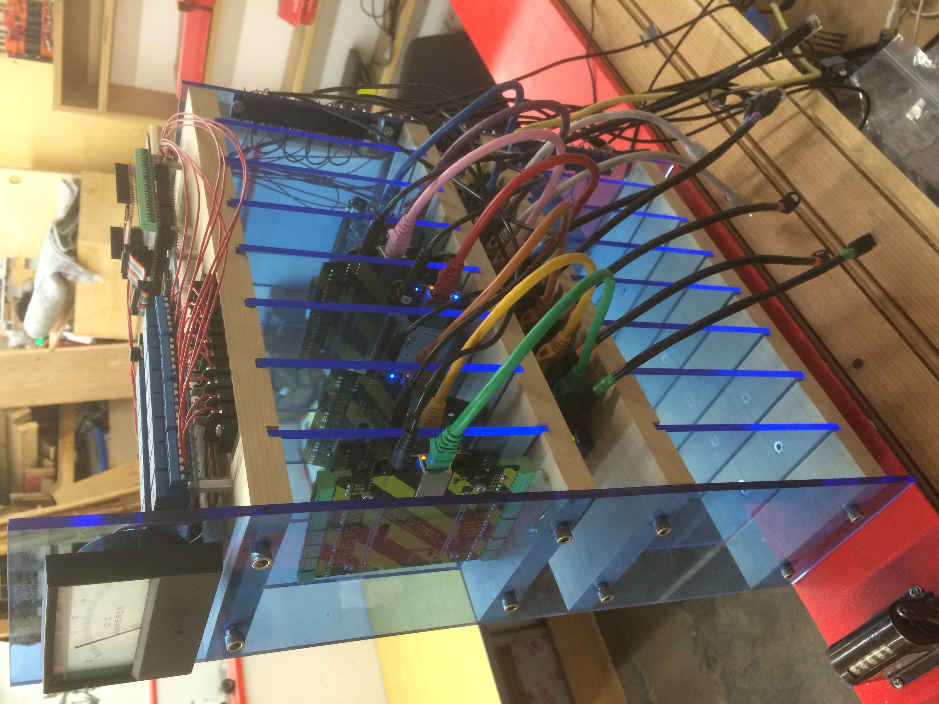
Revision 3: in which lasers are fired at acrylic

For the third revision, I switched to a hybrid wood-acrylic architecture. The dividers are Chemcast GP blue 2069 acrylic, 1/4" thick, from Delvie's Plastics.

To make the slots in the shelves precise, I built a dado sled with a small steel pin pressed through its face. As each slot was cut, the pin fit snugly into the previous slot. This proved highly repeatable, so the slots were finally spaced properly. Here's the sled after I cut all the shelves. You can see the pin near the blade slot.

Here's the first shelf getting slotted.

Here's the final assembly. The socket head cap screws on the ends are threaded into threaded inserts; getting those positioned with their axes perpendicular to the board ends was difficult. Before insertion, I chamfered the holes so that the inserts wouldn't tear up the board surface as the first threads bit in.

I also added a vintage analog current meter, so I could tell at a glance that the Rascals were cranking (each board uses around 0.250 mA).

Preliminary kernel test results

I haven't gathered good statistical data yet, but with the time I have spent testing Rascals in between Rascalfarm revisions, I figured out one significant fact: there was a significant bug in the Linux kernel that affected the reliability of the Beaglebone Black (and anything based on it, like the Rascal) for several months in 2014.

The problem was that, for some kernels in the 3.9-3.18 range, the USB OTG driver could screw up the board's power management system. The power management system (AKA the PMIC, "power management integrated circuit") watches the USB port to see if 5 V power is available. If it sees 5 V, it switches to that as a power source. Unfortunately, the USB OTG driver periodically pulsed the 5 V USB line high as a means of detecting whether a USB device had been plugged in. Occasionally, if the PMIC checked for 5 V at the same time, this short pulse was enough to fool it. The PMIC tried to switch to USB power just as the pulse ended. This resulted in the board power dropping, which caused a reboot. In my experience, this happened within minutes of booting and sometimes not for 18 hours.

You can follow the adventure as this was unraveled on the Beaglebone mailing list. It was a gentleman in the UK, Terry Barnaby, who finally cracked it, so far as I can tell.

The conclusion of all this is that if you want a reliable Beaglebone Black kernel, use something from:

• the 3.8.x series (currently the default shipping from Adafruit)
• 3.14.23-ti-r33 or later
• 3.18-rc4 or later

OK, back to programming.

Rascal 2: second prototype

Most of my time in the last few months has been devoted to developing the radiation monitoring system mentioned in the last post, but in the gaps, I've made some progress on the Rascal 2. The image below shows what is mostly a mechanical prototype. The bottom PCB is nearly identical to the first prototype, but with the accidentally rotated connectors fixed. The top PCB is really just a copy of the first PCB cut down with a jump shear so I could check the mechanical fit of various components.

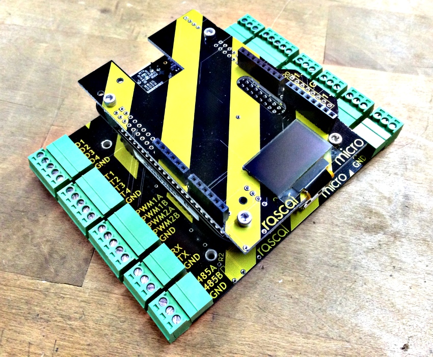
It's proving surprisingly difficult to join two stacked PCBs mechanically and electrically in a reliable, cheap, and compact fashion.

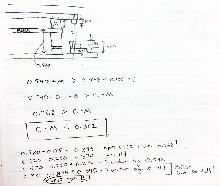
The specific problem that I ran into is that the male pins and threaded inserts that I want to use step 0.125" between sizes, but to seat the pins reliably in their sockets, I want their tips positioned vertically within a range of a 0.050" or so. The best match I could find raises the top PCB up quite far (0.375") and then uses long pins to reach back down to the lower PCB. The positioning is great, but it makes the whole system huge.

Here's the mechanical prototype. The aluminum hex standoff is the part marked "M" in the drawing above. The exposed metal pins are marked "C".

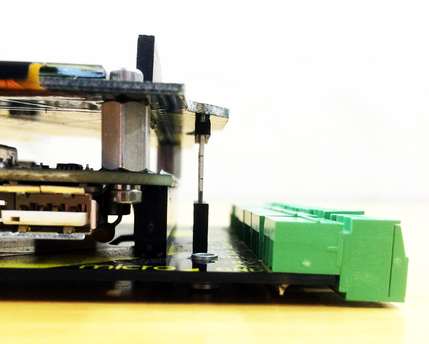
Overall, this is good progress-- the connectors look like they'll work, even if the whole stack is taller than I would like.