Homemade edging tool

Yesterday, I welded up an edging tool for making the grass along our sidewalk conform to my strict straightness requirements. I had been using it for 15 or 20 minutes before I realized that using an edging tool on your grass borders on the neurotic, and making your own edging tool is even weirder. But, I had already made it, and it came out pretty well, so here are some pictures.

The handle and the blue steel yoke come from the failed edger that I had, which clogged with grass and dirt almost instantaneously.

Pictures of the construction process are on Flickr.

The garden, after a savage edging:

Evaluating renewable energy companies

As part of my job at GreenMountain, I work with a lot of renewable energy startups. As a result, my friends are constantly telling me about new startups that they're excited about. This often leads to a discussion of how I evaluate renewable energy companies. The companies that my friends think are on the way to the top are rarely the ones that I think will win, so I think I should try to explain myself.

First off, my goal is to predict whether the company at hand will be able to produce huge amounts of energy from renewable sources at prices that rival fossil fuels. In most of the world, this is not currently possible-- fossil fuels are still cheap. There are regional exceptions, like residential solar power in ridiculously sunny places like the American southwest, but generally, no renewable energy company has yet succeeded.

Thus, the interesting question is: what do you need to do to win?

You must scale to huge.

A few years ago, I worked at an environmental foundation in Maine. For the last 8 years, the foundation has produced their own biodiesel from excess frialator oil from two nearby seafood restaurants that boomed in the summer. While I worked there, I was able to buy biodiesel for my Passat at whatever price the local gas station was charging for regular diesel.

It was brilliant, but the only reason it worked was that we got the frialator oil for free. I personally burned around 10% (50 gallons) of the annual biodiesel yield from the two seafood restaurants. I was driving fewer miles than the national average, and in a 42 mpg car. It's still a great idea, but biodiesel from frialator oil will never scale to huge.

Breakthroughs in the lab are not enough.

Every few weeks, I hear news of a breakthrough in solar cell technology in a laboratory setting. Usually, it's the Grätzel cell again. If not, it's often a new manufacturing technique that is purported to be cheap in high volume, but which is currently being produced in very low volume. Even the largest cell producers don't have a good idea of how cheap their cells will be when they scale beyond GW levels. (Maybe they're pretty good at 10 GW, but that's pushing it.) Claiming to be able to make those predictions accurately when you're below 1 kW is not credible.

You will not challenge Vestas soon.

In the more established renewable industries, like big wind, there are just a few players. Vestas, for example, sells about 25% of the large wind turbines in the world. They have around 20,000 employees and have been producing turbines for 30 years. They do over €1 BN in sales per quarter. Designing a MW-scale turbine takes years, never mind testing.

Most startups could not fit one large turbine blade in their offices. If you're a big wind startup with a plan to compete on that scale in the next few years, you are not credible. You might be able to do it, but you need a ten year plan.

Higher efficiency at higher cost is not an automatic win.

In small wind, a common approach is the shrouded wind turbine. The general idea is to add a shroud around the wind turbine that channels wind into the blades. So far, nobody has been successful with this approach-- the economics dictate that the marginal cost of blade extension beats that of shrouding. This is not to say that shrouded turbines will always lose, just that so far, nobody has been able to get an increase in efficiency that outweighs the increase in cost.

Concentrating photovoltaic systems face the same problem-- can you add a concentrating mirror cheaply enough that it's worth the cost? The jury is still out on that one.

Lower cost with lower efficiency is not an automatic win.

For years, solar cell companies have been trying to make "thin film" solar cells, i.e. cells that are manufactured by depositing a coating a few microns thick on a substrate, usually metal. Because thin film cells are so thin, they use very little material, so they're much cheaper per unit of area than conventional cells. Unfortunately, they're also less efficient. In the long run, thin film cells may still win, but so far it seems that, despite massive investments in R&D, the efficiency penalty outweighs the cost savings.

Every engineering challenge comes with a counterpart in marketing.

To win in renewable energy, you can't be just a brilliant engineer. You also need a team that can sell your products. It's like preventing car theft-- it doesn't do any good to lock one door of your car, even if you lock it really carefully, and the lock is really strong. You have to lock all the doors, every time you leave the car. In the same vein, your heat recovery system may be brilliant, but if you marketing efforts look amateurish, you're sunk.

The ocean, sun, wind, and rain are harsh.

Most energy systems have to survive outside for their ~20 year lifetime. If they can't, you have lost. Ocean power systems, for example, have to survive scouring from ice and abuse from drifting trees. Wind turbines have to survive hurricanes; solar panels must endure hail. If you're a slippery businessman, you might be able to sell a product good enough to give you 5 years to change your identity and escape to a country missing the requisite extradition treaty, but that won't solve our energy problem.

Please note in the comments respectable axes of evaluation that I have omitted.

Calculating solar panel shading in Python

Eventually, I'd like to install solar panels on our house, but I want to know that it will be worth it before I commit the money. Back in 2007, I wrote a library for calculating the path of the sun given the time and your location on the earth. Since then, I've been thinking about the next step, which is calculating how much neighboring houses and trees would obstruct the sun at different times of the day. In a nutshell, I wanted to replicate the calculations performed by devices like the Solmetric Suneye without paying $1500 for the device. To do the job right, I still need a quality circular fisheye lens ($680 new), but I've got a first approximation working with a $13 door peephole from McMaster.

(I do realize that I could just get a solar contractor to do all the site evaluation for me for free. That misses the point. If all I wanted was some sort of fiscal efficiency, I'd get a job as a financial executive or maybe something different from that, like a bank robber.)

Back to the task at hand.

Below is the image I started with, which I took back in the fall, before the leaves fell off the trees. This was using a Canon SD450 camera and the aforementioned peephole. I didn't take particular care to level the camera or center the peephole.

Using the Python Imaging Library, I cropped the photo to be square and switched to black and white mode. Then I mapped concentric rings in the image below to the subsequent straightened image.

Here's the straightening code. The guts are in the nested for loops near the end. (If there are any Pythonistas out there who know how to iterate over concentric rings using a list comprehension or map(), please let me know. The code below is functional and reasonable clear, but a little slow.)

```(lang=python)

Code under GPLv3; see pysolar.org for complete version.

def despherifyImage(im): (width, height) = im.size half_width = im.size[0]/2 half_height = im.size[1]/2 inpix = im.load() out = Image.new("L", (width, half_height)) outpix = out.load() full_circle = 1000.0 * 2 * pi for r in range(half_width): for theta in range(int(full_circle)): (inx, iny) = (round(r * cos(theta/1000.0)) + half_width, round(r * sin(theta/1000.0)) + half_width) (outx, outy) = (width - width * (theta/full_circle) - 1, r) outpix[outx, outy] = inpix[inx, iny] return out

```

The straightening works pretty well, but there is a little distortion that I think is caused by the peephole not being a perfectly spherical lens. Also, because the peephole is not centered on the camera lens, my concentric ring transformation isn't centered either.

From here, I needed to figure out where the sky ends and the buildings or trees start. Unfortunately, the buildings and trees are both lighter and darker than the sky in different places, so I can't just look for one type of transition. To detect the edge, I scan down each column of pixels and calculate the difference in darkness between consecutive pixels, ignoring whether the change was from light to dark or the reverse. The image below shows those differences, amplified by 10x to increase the contrast. The mathematicians call this calculation a finite forward difference.

Here's the finite difference code.

``` (lang=python)

Code under GPLv3; see pysolar.org for complete version.

def differentiateImageColumns(im): (width, height) = im.size pix = im.load() for x in range(width): for y in range(height - 1): pix[x, y] = min(10 * abs(pix[x, y] - pix[x, y + 1]), 255) return im

```

The last step is to scan down each column looking for the first large value. The first change that crosses a threshold is recorded. The final output is an array of values that measure the angle of the highest obstruction as a function of direction. As a sanity check, I drop a red dot on each value. It's hard to make out in the thumbnail below, but if you click on the image below, you'll get a larger version where you can see the red dots work pretty well.

I think the next step will be to calculate the total energy delivered per year using Pysolar.

Here's the full code.

``` (lang=python)

Code under GPLv3; see pysolar.org for complete version.

from PIL import Image from math import * import numpy as np

def squareImage(im): (width, height) = im.size box = ((width - height)/2, 0, (width + height)/2, height) return im.crop(box)

def despherifyImage(im): (width, height) = im.size half_width = im.size[0]/2 half_height = im.size[1]/2 inpix = im.load() out = Image.new("L", (width, half_height)) outpix = out.load() full_circle = 1000.0 * 2 * pi for r in range(half_width): for theta in range(int(full_circle)): (inx, iny) = (round(r * cos(theta/1000.0)) + half_width, round(r * sin(theta/1000.0)) + half_width) (outx, outy) = (width - width * (theta/full_circle) - 1, r) outpix[outx, outy] = inpix[inx, iny] return out

def differentiateImageColumns(im): (width, height) = im.size pix = im.load() for x in range(width): for y in range(height - 1): pix[x, y] = min(10 * abs(pix[x, y] - pix[x, y + 1]), 255) return im

def redlineImage(im): (width, height) = im.size pix = im.load() threshold = 300 for x in range(width): for y in range(height - 1): (R, G, B) = pix[x, y] if R + G + B > threshold: pix[x, y] = (255, 0, 0) break return im

im = Image.open('spherical.jpg').convert("L") im = squareImage(im)

lin = despherifyImage(im) d = differentiateImageColumns(lin).convert("RGB") r = redlineImage(d)

r.show()

```

Least squares polynomial fitting in Python

A few weeks ago at work, in the course of reverse engineering a dissolved oxygen sensor calibration routine, Jon needed to fit a curve to measured data so he could calculate calibration values from sensor readings, or something like that. I don’t know how he did the fitting, but it got me thinking about least squares and mathematical modeling.

The tools I’ve used for modeling (Matlab, Excel and the like) and the programming languages I’ve used for embedded systems (C and Python, mostly) are disjoint sets. Who wants to use Matlab for network programming, when you could use Python instead? Who wants to use C for calculating eigenvalues, when you could use Matlab instead? Generally, nobody.

Unfortunately, sometimes you need to do both in the same system. I’m not sure that I’m making a wise investment, but I think that Python’s numerical libraries have matured enough that Python can straddle the divide.

So, here’s what I’ve figured out about least squares in Python. My apologies to most of you regular readers, as you will find this boring as hell. This one’s for me and the internet.

Least squares estimation

Generally, least squares estimation is useful when you have a set of unknown parameters in a mathematical model. You want to estimate parameters that minimize the errors between the model and your data. The canonical form is:

Ax=y where:

* A is an M \times N full rank matrix with M > N (skinny)
* x is a vector of length N
* y is a vector of length M

As matrices, this looks like

You want to minimize the L2-norm, ||Ax-y||. To be explicit, this means that if you define the residuals r = Ax - y, you want to choose the that minimizes \sqrt{r_1^2 + ... r_M^2}. This is where the “least squares” name comes from– you’re going to choose the that results in the squares of r being least.

Once you know A and y, actually finding the best x (assuming you have a computer at your disposal) is quick. The derivation sets the gradient of ||r||^2 with respect to x to zero and then solves for x. Mathematicians call the solution the Moore-Penrose pseudo-inverse. I call it “what the least squares function returned.” In any case, here it is:

Fortunately, one need not know the correct name and derivation of a thing for it to be useful.

So now, how do you go about using this technique to fit a polynomial to some data?

Polynomial fitting

In the case of polynomial fitting, let’s say you have a series of data points, (t_i, y_i) that you got from an experiment. The t_i are the times at which you made your observations. Each y_i is the reading from your sensor that you noted at the time with the same i.

Now you want to find a polynomial y = f(t) that approximates your data as closely as possible. The final output will look something like

where you have cleverly chosen the x_i for the best fit to your data. You’ll be able to plug in whatever value of t you want and get an estimate of y in return.

In the conventional form, we are trying to find an approximate solution to Ax=y

In this case, A is called the Vandermonde matrix; it takes the form:

(This presumes that you want to use powers of t as your basis functions– not a good idea for all modeling tasks, but this blog post is about polynomial fitting. Another popular choice is sinusoidal functions; perhaps Google can tell you more on that topic.)

(Also, the Vandermonde matrix is sometimes defined with the powers ascending from left to right, rather than descending. Descending works better with Python because of the coefficient order that numpy.poly1d() expects, but mathematically either way works.)

(Back to polynomial fitting.)

Each observation in your experiment corresponds to a row of A; A_i * x = y_i. Presumably, since every experiment has some noise in it, there is no x that fits every observation exactly. You know all the t_i, so you know A.

As a reminder, our model looks like this:

You can check that A makes sense by imagining the matrix multiplication of each row of A with x to equal the corresponding entry in y. For the second row of A, we have y_2 = x_Nt_2 + . . . + x_2t_2^2 + x_1t_2^1 + x_0

which is just the polynomial we’re looking to fit to the data.

Now, how can we actually do this in Python?

Python code

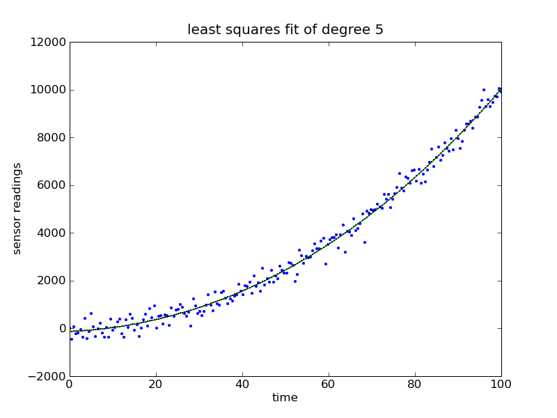
Let’s suppose that we have some data that looks like a noisy parabola, and we want to fit a polynomial of degree 5 to it. (I chose 5 randomly; it’s a stupid choice. More on selection of polynomial degree in another post.)

```(lang=python) import numpy as np import scipy as sp import matplotlib.pyplot as plt

degree = 5

generate a noisy parabola

t = np.linspace(0,100,200) parabola = t**2 noise = np.random.normal(0,300,200) y = parabola + noise ```

So now we have some fake data– an array of times and an array of noisy sensor readings. Next, we form the Vandermonde matrix and find an approximate solution for x. Note that numpy.linalg.lstsq() returns a tuple; we’re really only interested in the first element, which is the array of coefficients.

``` (lang=python)

form the Vandermonde matrix

A = np.vander(t, degree)

find the x that minimizes the norm of Ax-y

(coeffs, residuals, rank, sing_vals) = np.linalg.lstsq(A, y)

create a polynomial using coefficients

f = np.poly1d(coeffs)

```

Three lines of code later, we have a solution!

I could have also used numpy.polyfit() in place of numpy.linalg.lstsq(), but then I wouldn’t be able to write a blog post about regularized least squares later.

Now we’ll plot the data and the fitted curve to see if the function actually works!

``` (lang=python)

for plot, estimate y for each observation time

y_est = f(t)

create plot

plt.plot(t, y, '.', label = 'original data', markersize=5) plt.plot(t, y_est, 'o-', label = 'estimate', markersize=1) plt.xlabel('time') plt.ylabel('sensor readings') plt.title('least squares fit of degree 5') plt.savefig('sample.png')

```

This post took two-thirds of eternity to write. Feel free to ask questions or point out how confused I am below.

Next: regularized least squares! Or maybe selection of polynomial degree! Or maybe forgetting the blog and melting brain with TV!